Temperature Example

Introduction

Gaussian processes are quite popular in geostatistics where models such as Kriging are used to interpolate spatial fields. The idea is very similar to the 1D Example, there is some unknown function (in our example it will be temperature as a function of location) and you have noisy observations of the function (from weather stations) which you would like to use to make estimates at new locations.

Temperature Data

For this example we’ll use the Global Summary of the Day (GSOD) data to produce an estimate of the average temperature for a given day over the continental United States (CONUS).

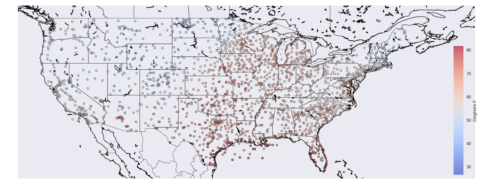
Here are the GSOD observation of average temperature for May 1st, 2018,

Temperature Model

We’re going to build our temperature model to incorporate the following priors about how temperature should be have.

• Temperature at neighboring locations should be similar.

• There is some non-zero average temperature.

• Temperature decreases with elevation

To accomplish this we can build a covariance function that is not dissimilar from the one used in the 1D Example. We can start with measurement noise,

IndependentNoise<Station> noise(2.0);

Which states that each weather station makes observations of the average temperature that includes noise with a standard deviation of \(2\) degrees.

We can then define a mean value for our field. In reality we might expect that the mean average temperature for a day would vary geographically, for this model we’ll simply claim that there is some mean average temperature for all of CONUS,

Constant mean;

Now we capture the spatial variation by saying that locations near each other in terms of great circle distance will be similar,

// The angular distance is equivalent to the great circle distance
SquaredExponential<StationDistance<AngularDistance>> angular_sqrexp;

Then add that stations at different elevations will be dissimilar,

// Radial distance is the difference in lengths of the X, Y, Z
// vectors, which translates into a difference in height so
// this term means "station at different elevations will be less correlated"
Exponential<StationDistance<RadialDistance>> radial_exp;

These can be combined to get our final covariance function,

auto spatial_cov = angular_sqrexp * radial_exp;
auto covariance = mean + noise + spatial_cov;

For the full implementation details see the example code.

Elevation Scaling

Then as we’d mentioned we’d like to include the concept of temperature decreasing with elevation. To do this we can create a scaling term which scales the mean value based on the elevation.

\[\mbox{elevation_scaling}(h) = 1. + \alpha \left(H - h\right)_{+}.\]

Where \(\left(\cdot\right)_{+}\) could also be written \(\mbox{max}(0, \cdot)\) and returns the argument if positive \(0\) otherwise. The resulting function will decrease at a rate of \(\alpha\) until \(h >= H\) afterwhich the scaling term will flatten out to a constant value of \(1\). By multiplying this term through with the mean we get a prior which will allow for higher temperatures at low elevations.

Here is how you can implement such a scaling function in albatross.

class ElevationScalingFunction : public albatross::ScalingFunction {
 public:

  ALBATROSS_DECLARE_PARAMS(elevation_scaling_center, elevation_scaling_factor);

  ElevationScalingFunction(double center = 1000., double factor = 3.5 / 300) {
    elevation_scaling_center = {center, UniformPrior(0., 5000.)};
    elevation_scaling_factor = {factor, PositivePrior()};
  };

  std::string get_name() const { return "elevation_scaled"; }

  double _call_impl(const Station &x) const {
    // This is the negative orientation rectifier function which
    // allows lower elevations to have a higher variance.
    const double center = elevation_scaling_center.values;
    const double factor = elevation_scaling_factor.value;
    return 1. + factor * fmax(0., (center - x.height));
  }
};

// Scale the constant temperature value in a way that defaults
// to colder values for higher elevations.
ScalingTerm<ElevationScalingFunction> elevation_scalar;
auto elevation_scaled_mean = elevation_scalar * mean;
auto covariance = elevation_scaled_mean + noise + spatial_cov;

Gridded Predictions

Now that we’ve defined the covariance function we can let albatross do the rest!

auto model = gp_from_covariance(covariance);
model.fit(data);
const auto predictions = model.predict(grid_locations);

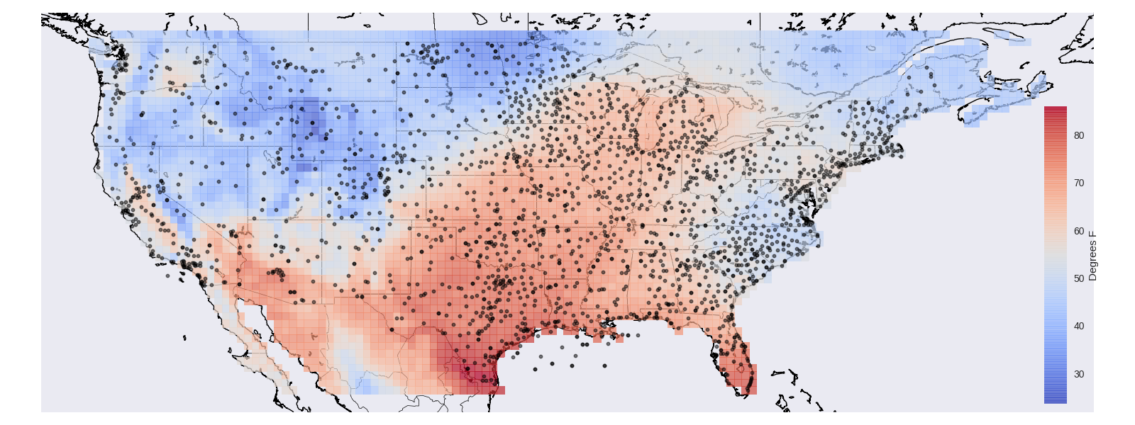
Here we created a Gaussian process from the covariance function, fit the model using the GSOD data and then made predictions on a grid. The predictions hold information about the mean and variance of the resulting estimates. We can look at the mean of the estimates,

and perhaps more interestingly we can also get out the variance, or how confident the model is about its predictions,

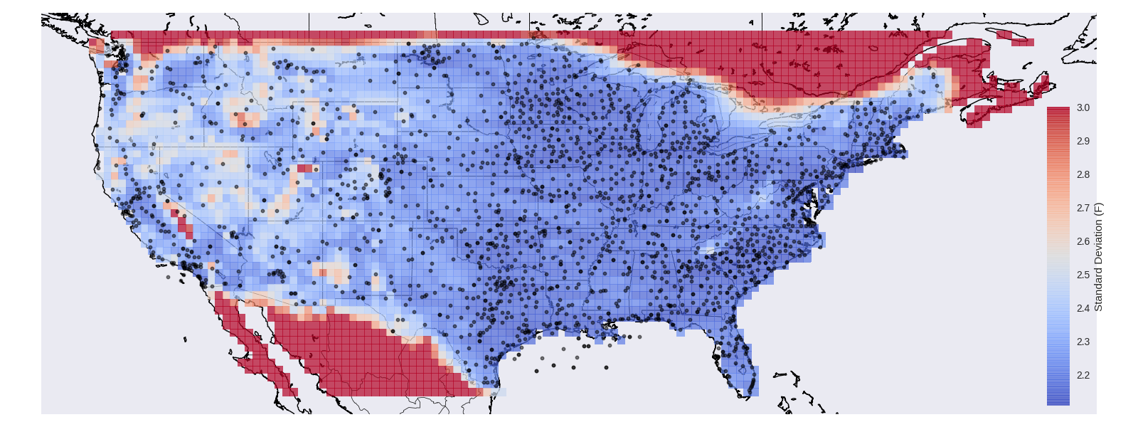
Notice that the model is capable of realizing that it’s estimates should be trusted less in mountainous regions!

If you want to run this on your own you can build the temperature_example target:

make temperature_example && ./examples/temperature_example -input ../examples/temperature_example/gsod.csv  -predict ../examples/temperature_example/prediction_locations.csv -thin 10 -output ./temperature_predictions.csv
python ../examples/temperature_example/plot_temperature_example.py ../examples/temperature_example/gsod.csv ./temperature_predictions.csv